KLH PEER MENTOR BLOG

BY T.AKSHITHA, S.PRAMOD

R Introduction

R is an open-source programming language that is widely used as a statistical software and data analysis tool. R generally comes with the Command-line interface. R is available across widely used platforms like Windows, Linux, and macOS. Also, the R programming language is the latest cutting-edge tool.

It was designed by Ross Ihaka and Robert Gentleman at the University of Auckland, New Zealand, and is currently developed by the R Development Core Team. R programming language is an implementation of the S programming language. It also combines with lexical scoping semantics inspired by Scheme. Moreover, the project conceives in 1992, with an initial version released in 1995 and a stable beta version in 2000.

Why R Programming Language?

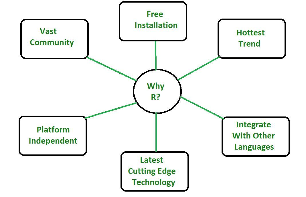
R programming is used as a leading tool for machine learning, statistics, and data analysis. Objects, functions, and packages can easily be created by R.
It’s a platform-independent language. This means it can be applied to all operating system.
It’s an open-source free language. That means anyone can install it in any organization without purchasing a license.
R programming language is not only a statistic package but also allows us to integrate with other languages (C, C++). Thus, you can easily interact with many data sources and statistical packages.
The R programming language has a vast community of users and it’s growing day by day.
R is currently one of the most requested programming languages in the Data Science job market that makes it the hottest trend nowadays.

Features of R Programming Language

Statistical Features of R:

Basic Statistics: The most common basic statistics terms are the mean, mode, and median. These are all known as “Measures of Central Tendency.” So using the R language we can measure central tendency very easily.
Static graphics: R is rich with facilities for creating and developing interesting static graphics. R contains functionality for many plot types including graphic maps, mosaic plots, biplots, and the list goes on.
Probability distributions: Probability distributions play a vital role in statistics and by using R we can easily handle various types of probability distribution such as Binomial Distribution, Normal Distribution, Chi-squared Distribution and many more.
Data analysis: It provides a large, coherent and integrated collection of tools for data analysis.

Programming Features of R:

R Packages: One of the major features of R is it has a wide availability of libraries. R has CRAN(Comprehensive R Archive Network), which is a repository holding more than 10, 0000 packages.
Distributed Computing: Distributed computing is a model in which components of a software system are shared among multiple computers to improve efficiency and performance. Two new packages ddR and multidplyr used for distributed programming in R were released in November 2015.

Programming in R:

Since R is much similar to other widely used languages syntactically, it is easier to code and learn in R. Programs can be written in R in any of the widely used IDE like R Studio, Rattle, Tinn-R, etc. After writing the program save the file with the extension .r. To run the program use the following command on the command line:

Advantages of R:

R is the most comprehensive statistical analysis package. As new technology and concepts often appear first in R.
As R programming language is an open source. Thus, you can run R anywhere and at any time.
R programming language is suitable for GNU/Linux and Windows operating system.
R programming is cross-platform which runs on any operating system.
In R, everyone is welcome to provide new packages, bug fixes, and code enhancements.

Disadvantages of R:

In the R programming language, the standard of some packages is less than perfect.
Although, R commands give little pressure to memory management. So R programming language may consume all available memory.
In R basically, nobody to complain if something doesn’t work.
R programming language is much slower than other programming languages such as Python and MATLAB.

Applications of R:

We use R for Data Science. It gives us a broad variety of libraries related to statistics. It also provides the environment for statistical computing and design.
R is used by many quantitative analysts as its programming tool. Thus, it helps in data importing and cleaning.
R is the most prevalent language. So many data analysts and research programmers use it. Hence, it is used as a fundamental tool for finance.
Tech giants like Google, Facebook, bing, Twitter, Accenture, Wipro and many more using R nowadays.

Optimization Methods

Here are five key methods for big data optimisation

Standardise data

Big data is large, complex and prone to errors, if not standardised correctly. There are many ways big data can turn out to be inaccurate, if not formatted properly. Take, for example, a naming format – Micheal Dixon can also be M. Dixon or Mike Dixon. An inconsistent format leads to several problems, like data duplication and skewered analytics results. Therefore, a vital part of big data optimisation is setting a standard format so that petabytes of data have a consistent format and the ability to generate more accurate results.

‘Tune-up’ algorithms

It is not just enough to implement algorithms that analyse and finetune your big data. There are several algorithms used to optimise big data, such as diagonal bundle method, convergent parallel algorithms and limited memory bundle algorithm. You need to make sure that the algorithms are fine-tuned to fit your organisation’s goals and objectives. Data analytics algorithms are responsible for sifting through big data to achieve objectives and provide value.

Remove latency in processing

Latency in processing refers to the delay (measured in milliseconds) when retrieving data from the databases. Latency hurts data processing because it hurts the rate you get results. In an age where data analytics offers real-time insights having delays in processing is simply unacceptable. To significantly reduce the delay in processing, organisations should move away from conventional databases and towards the latest technology, like in-memory processing.

Identify and fix errors

A key part of big data optimisation is fixing broken data. You can have fine-tuned algorithms and install the best analytics platforms, but it does not mean anything if the data is not accurate. If the data is incorrect, it leads to inaccurate findings, which hurts your ROI. In such cases, a data analyst will have to go in and fix data to make sure everything is accurate. Big data can have plenty of errors, like duplicated entries, inconsistent formats, incomplete information and even inaccurate data. In such cases, data analysts have to use various tools, like data deduplication tools to identify and fix errors.

Eliminate unnecessary data

Not all data collected is relevant to your organisation’s objectives as bloated data bogs down algorithms and slows down the rate of processing. Hence, a vital part of big data optimisation is to eliminate unnecessary data. Once unnecessary information is eliminated it increases the rate of data processing and optimises big data.

Leverage the latest technology

Data analytics is constantly evolving and it is important to keep up with the latest technology. Recent technological developments, like AI and machine learning, make big data optimisation easier and improves the quality of work. For example, AI paves the way for a host of new technologies, like natural language processing that helps machines process human language and sentiment. Investing in the latest technology improves big data optimisation because it accelerates the process while reducing the chances of errors.

Bringing it all together

Big data optimisation is the key to accurate data analytics. If data is not properly optimised, it leads to several problems, like inaccurate findings and delays in processing. However, there are at least six different ways to optimise big data. These methods including standardising format, tuning algorithms, leveraging the latest technology, fixing data errors and removing any latency in processing. If data is optimised, it improves the rate of data processing and the accuracy of results.

Introduction to Blind Search

Introduction

A blind search (also called an uninformed search) is a search that has no information about its domain. The only thing that a blind search can do is distinguish a non-goal state from a goal state.

Consider the following, simplified map of Romania

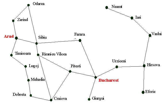
Assume you are currently in Arad and we want to get to Bucharest. If we produce a search tree, level 1 will have three states; Zerind, Sibiu and Timisoara. A blind search will have no preference as to which node it should explore first (later we will see that we can develop search strategies that incorporate some intelligence).

You may wonder why we should use a blind search, when we could use a search with some built in intelligence. The simple answer is that there may not be any information we can use. We might just be looking for an answer and won't know we've found it until we see it.
But it is also useful to study these uninformed searches as they form the basis for some of the intelligent searches that we shall be looking at later.

The blind searches we are about to consider only differ in the order in which we expand the nodes but, as we shall see, this can have a dramatic effect as to how well the search performs.

Breadth-First Search

Using a breadth-first strategy we expand the root level first and then we expand all those nodes (i.e. those at level 1) before we expand any nodes at level 2.
Or to put it another way, all nodes at level d are expanded before any nodes at level d+1.
In fact, if you (as suggested) worked through the search algorithm shown on an earlier slide set (Formulation) you will have seen a breadth first search in action.
This is because we can implement a breadth first search by using a queuing function that adds expanded nodes to the end of the queue.
Therefore, we could implement a breadth-first search using the following algorithm

Function BREADTH-FIRST-SEARCH(problem) returns a solution or failure
Return GENERAL-SEARCH(problem, ENQUEUE-AT-END)

Look at the animated powerpoint presentation to see breadth first search in action (go back to the Outline) and click the appropriate link there)

We can make the following observations about breadth-first searches

It is a very systematic search strategy as it considers all nodes (states) at level 1 and then all states at level 2 etc.
If there is a solution breadth first search is guaranteed to find it.
If there are several solutions then breadth first search will always find the shallowest goal state first and if the cost of a solution is a non-decreasing function of the depth then it will always find the cheapest solution.

You will recall that we defined four criteria that we are going to use to measure various search strategies; these being completeness, time complexity, space complexity and optimality. In terms of those, breadth-first search is both complete and optimal. Or rather, it is optimal provided that the solution is also the shallowest goal state or, to put it another way, the path cost is a function of the depth.

But what about time and space complexity?

To measure this we have to consider the branching factor, b; that is every state creates b new states.
The root of our tree has 1 state. Level 1 produces b states and the next level produces b² states. The next level produces b³ states.
Assuming the solution is found a level d then the size of the tree is

1 + b + b² + b³ + ... + b^d

(Note : as the solution could be found at any point on the d level then the search tree could be smaller than this).

This type of exponential growth (i.e. O(b^d) ) is not very healthy. You only have to look at the following table to see why.

Depth	Nodes	Time	Memory
0	1	1 millisecond	100 kbytes
2	111	0.1 second	11 kilobytes
4	11,111	11 seconds	1 megabyte
6	10⁶	18 minutes	111 megabytes
8	10⁸	31 hours	11 gigabytes
10	10¹⁰	128 days	1 terabyte
12	10¹²	35 years	111 terabytes
14	10¹⁴	3500 years	11,111 terabytes

Time and memory requirements for breadth-first search, assuming a branching factor of 10, 100 bytes per node and searching 1000 nodes/second

We can make some observations about these figures

Space is more of a factor to breadth first search than time. If you care about the answer you would probably be happy to wait for 31 hours for an answer to a level 8 problem but you are unlikely to have the 11 gigabytes of space that is needed to complete the search.
But time is still an issue. Who has 35 years to wait for an answer to a level 12 problem (or even 128 days to a level 10 problem).
We could argue that as technology gets faster then the type of problems shown above will be solvable. That is true, but even if technology is 100 times faster we would still have to wait 35 years for a level 14 problem and what if we hit a level 15 problem!

It is true to say that breadth first search can only be used for small problems. If we have larger problems to solve then there are better blind search strategies that we can try.

Uniform Cost Search

We have said that breadth first search finds the shallowest goal state and that this will be the cheapest solution so long as the path cost is a function of the depth of the solution. But, if this is not the case, then breadth first search is not guaranteed to find the best (i.e. cheapest) solution.
Uniform cost search remedies this.
It works by always expanding the lowest cost node on the fringe, where the cost is the path cost, g(n). In fact, breadth first search is a uniform cost search with g(n) = DEPTH(n).

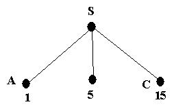
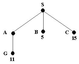
Consider the following problem.

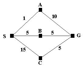
We wish to find the shortest route from S to G; that is S is the initial state and G is the goal state. We can see that SBG is the shortest route but if we let breadth first search loose on the problem it will find the path SAG; assuming that A is the first node to be expanded at level 1.
But this is how uniform cost search tackles the problem.

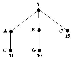
We start with the initial state and expand it. This leads to the following tree

The path cost of A is the cheapest, so it is expanded next; giving the following tree

We now have a goal state but the algorithm does not recognize it yet as there is still a node with a cheaper path cost. In fact, what the algorithm does is order the queue by the path cost so the node with cost 11 will be behind node B in the queue.
Node B (being the cheapest) is now expanded, giving

A goal state (G) will now be at the front of the queue. Therefore the search will end and the path SBG will be returned.

Look at the animated powerpoint presentation to see uniform cost search in action (go back to the Outline and click the appropriate link there)

In summary, uniform cost search will find the cheapest solution provided that the cost of the path never decreases as we proceed along the path. If this requirement is not met then we never know when we will meet a negative cost. The result of this would be a need to carry out an exhaustive search of the entire tree.

Depth-First Search

Depth first search explores one branch of a tree before it starts to explore another branch. It can be implemented by adding newly expanded nodes at the front of the queue.

Using the general search algorithm we can implement it as follows.

Function DEPTH-FIRST-SEARCH(problem) returns a solution or failure
Return GENERAL-SEARCH(problem, ENQUEUE-AT-FRONT)

Pictorially, a depth first search can be shown as follows

Look at the animated powerpoint presentation to see depth first search in action (go back to the Outline and click the appropriate link there)

We can make the following comments about depth first search

It has modest memory requirements. It only needs to store the path from the root to the leaf node as well as the unexpanded nodes. For a state space with a branching factor of b and a maximum depth of m, depth first search requires storage of bm nodes.
The time complexity for depth first search is b^m in the worst case.
If depth first search goes down a infinite branch it will not terminate if it does not find a goal state. If it does find a solution there may be a better solution at a higher level in the tree. Therefore, depth first search is neither complete nor optimal.

Depth-Limited Search

The problem with depth first search is that the search can go down an infinite branch and thus never return.
Depth-limited search avoids this problem by imposing a depth limit which effectively terminates the search at that depth.
The algorithm can be implemented using the general search algorithm by using operators to keep track of the depth.

The choice of the depth parameter can be an important factor. Choosing a parameter that is too deep is wasteful in terms of both time and space. But choosing a depth parameter that is too shallow may result in never reaching a goal state.

As long as the depth parameter, l (this is lower case L, not the digit one), is set "deep enough" then we are guaranteed to find a solution if it exists. Therefore it is complete as long as l >= d (where d is the depth of the solution). If this condition is not met then depth limited search is not complete.

The space requirements for depth limited search are similar to depth first search. That is, O(bl).
The time complexity is O(b^l )

Iterative Deepening Search

The problem with depth limited search is deciding on a suitable depth parameter. If you look at the Romania map you will notice that there are 20 towns. Therefore, any town is reachable from any other town with a maximum path length of 19.
But, closer examination reveals that any town is reachable in at most 9 steps. Therefore, for this problem, the depth parameter should be set as 9. But, of course, this is not always obvious and choosing a parameter is one reason why depth limited searches are avoided.

To overcome this problem there is another search called iterative deepening search.
This search method simply tries all possible depth limits; first 0, then 1, then 2 etc., until a solution is found.
What iterative deepening search is doing is combining breadth first search and depth first search.

Look at the animated powerpoint presentation to see iterative deepening search in action (go back to the Outline and click the appropriate link there)

It may appear wasteful as it is expanding nodes multiple times. But the overhead is small in comparison to the growth of an exponential search tree.
To show this is the case, consider this.

For a depth limited search to depth d with branching b the number of expansions is

1 + b + b² + … + b^d-2 + b^d-1 + b^d

If we apply some real numbers to this (say b=10 and d=5), we get

1 + 10 + 100 + 1,000 +10,000 + 100,000 = 111,111

For an iterative deepening search the nodes at the bottom level, d, are expanded once, the nodes at d-1 are expanded twice, those at d-3 are expanded three times and so on back to the root.
The formula for this is

(d+1)1 + (d)b+(d-1)b² + … + 3b^d-2 + 2b^d-1 + 1b^d

If we plug in the same numbers we get

6 + 50 + 400 + 3,000 + 20,000 + 100,000 = 123,456

You can see that, compared to the overall number of expansions, the total is not substantially increased.

In fact, when b=10 only about 11% more nodes are expanded for a breadth first search or a depth limited node down to level d.
Even when the branching factor is 2 iterative deepening search only takes about twice as long as a complete breadth first search.

The time complexity for iterative deepening search is O(b^d) with the space complexity being O(bd).

For large search spaces where the depth of the solution is not known iterative deepening search is normally the preferred search method.

Checking for Repeated States

In this section we have looked at five different blind search algorithms. Whilst these algorithms are running it is possible (and for some problems extremely likely) that the same state will be generated more than once.
If we can avoid this then we can limit the number of nodes that are created and, more importantly, stop the need to have to expand the repeated nodes.

There are three methods we can use to stop generating repeated nodes.

Do not generate a node that is the same as the parent node. Or, to put it another way, do not return to the state you have just come from.
Do not create paths with cycles in them. To do this we can check each ancestor node and refuse to create a state that is the same as this set of nodes.
Do not generate any state that is the same as any state generated before. This requires that every state is kept in memory (meaning a potential space complexity of O(b^d)).

The three methods are shown in increasing order of computational overhead in order to implement them.
The last one could be implemented via hash tables to make checking for repeated states as efficient as possible.

Simulated Annealing algorithm

Simulated annealing (SA) is a probabilistic technique for approximating the global optimum of a given function. Specifically, it is a metaheuristic to approximate global optimization in a large search space for an optimization problem. It is often used when the search space is discrete (for example the traveling salesman problem, the boolean satisfiability problem, protein structure prediction, and job-shop scheduling). For problems where finding an approximate global optimum is more important than finding a precise local optimum in a fixed amount of time, simulated annealing may be preferable to exact algorithms such as gradient descent or branch and bound.

The name of the algorithm comes from annealing in metallurgy, a technique involving heating and controlled cooling of a material to alter its physical properties. Both are attributes of the material that depend on their thermodynamic free energy. Heating and cooling the material affects both the temperature and the thermodynamic free energy or Gibbs energy. Simulated annealing can be used for very hard computational optimization problems where exact algorithms fail; even though it usually achieves an approximate solution to the global minimum, it could be enough for many practical problems.

The problems solved by SA are currently formulated by an objective function of many variables, subject to several constraints. In practice, the constraint can be penalized as part of the objective function.

Similar techniques have been independently introduced on several occasions, including Pincus (1970),^[1] Khachaturyan et al (1979,^[2] 1981^[3]), Kirkpatrick, Gelatt and Vecchi (1983), and Cerny (1985).^[4] In 1983, this approach was used by Kirkpatrick, Gelatt Jr., Vecchi,^[5] for a solution of the traveling salesman problem. They also proposed its current name, simulated annealing.

This notion of slow cooling implemented in the simulated annealing algorithm is interpreted as a slow decrease in the probability of accepting worse solutions as the solution space is explored. Accepting worse solutions allows for a more extensive search for the global optimal solution. In general, simulated annealing algorithms work as follows. The temperature progressively decreases from an initial positive value to zero. At each time step, the algorithm randomly selects a solution close to the current one, measures its quality, and moves to it according to the temperature-dependent probabilities of selecting better or worse solutions, which during the search respectively remain at 1 (or positive) and decrease towards zero.

The simulation can be performed either by a solution of kinetic equations for density functions^[6]^[7] or by using the stochastic sampling method.^[5]^[8] The method is an adaptation of the Metropolis–Hastings algorithm, a Monte Carlo method to generate sample states of a thermodynamic system, published by N. Metropolis et al. in 1953.^[9]

Simulated Annealing is a stochastic global search optimization algorithm.

The algorithm is inspired by annealing in metallurgy where metal is heated to a high temperature quickly, then cooled slowly, which increases its strength and makes it easier to work with.

The annealing process works by first exciting the atoms in the material at a high temperature, allowing the atoms to move around a lot, then decreasing their excitement slowly, allowing the atoms to fall into a new, more stable configuration.

When hot, the atoms in the material are more free to move around, and, through random motion, tend to settle into better positions. A slow cooling brings the material to an ordered, crystalline state.

The simulated annealing optimization algorithm can be thought of as a modified version of stochastic hill climbing.

Stochastic hill climbing maintains a single candidate solution and takes steps of a random but constrained size from the candidate in the search space. If the new point is better than the current point, then the current point is replaced with the new point. This process continues for a fixed number of iterations.

Simulated annealing executes the search in the same way. The main difference is that new points that are not as good as the current point (worse points) are accepted sometimes.

A worse point is accepted probabilistically where the likelihood of accepting a solution worse than the current solution is a function of the temperature of the search and how much worse the solution is than the current solution.

The algorithm varies from Hill-Climbing in its decision of when to replace S, the original candidate solution, with R, its newly tweaked child. Specifically: if R is better than S, we’ll always replace S with R as usual. But if R is worse than S, we may still replace S with R with a certain probability

The initial temperature for the search is provided as a hyperparameter and decreases with the progress of the search. A number of different schemes (annealing schedules) may be used to decrease the temperature during the search from the initial value to a very low value, although it is common to calculate temperature as a function of the iteration number.

A popular example for calculating temperature is the so-called “fast simulated annealing,” calculated as follows

temperature = initial_temperature / (iteration_number + 1)

We add one to the iteration number in the case that iteration numbers start at zero, to avoid a divide by zero error.

The acceptance of worse solutions uses the temperature as well as the difference between the objective function evaluation of the worse solution and the current solution. A value is calculated between 0 and 1 using this information, indicating the likelihood of accepting the worse solution. This distribution is then sampled using a random number, which, if less than the value, means the worse solution is accepted.

It is this acceptance probability, known as the Metropolis criterion, that allows the algorithm to escape from local minima when the temperature is high.

This is called the metropolis acceptance criterion and for minimization is calculated as follows:

criterion = exp( -(objective(new) – objective(current)) / temperature)

Where exp() is e (the mathematical constant) raised to a power of the provided argument, and objective(new), and objective(current) are the objective function evaluation of the new (worse) and current candidate solutions.

The effect is that poor solutions have more chances of being accepted early in the search and less likely of being accepted later in the search. The intent is that the high temperature at the beginning of the search will help the search locate the basin for the global optima and the low temperature later in the search will help the algorithm hone in on the global optima.

The temperature starts high, allowing the process to freely move about the search space, with the hope that in this phase the process will find a good region with the best local minimum. The temperature is then slowly brought down, reducing the stochasticity and forcing the search to converge to a minimum

Introduction to Tabu Search

Tabu Search is a commonly used meta-heuristic used for optimizing model parameters. A meta-heuristic is a general strategy that is used to guide and control actual heuristics. Tabu Search is often regarded as integrating memory structures into local search strategies. As local search has a lot of limitations, Tabu Search is designed to combat a lot of those issues.

Tabu Search (TS)

The basic idea of Tabu Search is to penalize moves that take the solution into previously visited search spaces (also known as tabu). Tabu Search, however, does deterministically accept non-improving solutions in order to prevent getting stuck in local minimums.

Short-term vs. Long-term Memory

Short Term memory is based off of recency of occurrence and is used to prevent the search algorithm from revisiting previously visited solutions and also can be used to return to good components in order to localize and intensify a search. This is accomplished by the Tabu List and is also known as intensification.

Long Term memory is based off of frequency of occurrence and is used to diversity the search and explore unvisited areas of the search space by avoiding explored areas. This is accomplished by frequency memory and is also known as diversification.

Tabu List

The Tabu List is the cornerstone of utilizing short-term memory. This list stores a fixed amount of recently made moves. In some implementations, complete solutions are used instead of the moves used but this is not ideal if complete solutions are very large due to space limitations. Some examples of these moves are:

swap nodes in a graph/tour
toggling a bit between 0 and 1
insert or delete edges in a graph

Tabu Tenure

The Tabu Tenure is the number of iterations that a move stays in the Tabu List. The moves that are in the Tabu List are moves that cannot be made again as it was already recently visited. There are two ways to implement the Tabu Tenure (T):

Static: choose T to be a constant (often sqrt(T))
Dynamic: choose T randomly between some T_min and T_max

Aspiration Criteria

This is an optional part of Tabu Search. Moves or solutions that are part of the Aspiration Criteria cancel out the Tabu and the move can be made even if it’s in the Tabu List. This can also be used to prevent stagnation in cases where all possible moves are prohibited by the Tabu List. Some examples of Aspiration Criteria are:

if the new solution is better than the current best solution, then the new solution is used even if it’s on the Tabu List
setting the Tabu Tenure to be a smaller value

Frequency Memory

This memory holds the total number of iterations that each solution was picked since the beginning of the search. Solutions that were visited more are less likely to to be picked again and would promote more diverse solutions. There are two main approaches for diversifying:

Restart Diversification: allows components that rarely appear to be in the current solution by restarting the search from these points
Continuous Diversification: biases the evaluation of possible moves with the frequency of these moves. Moves that do not appear as often will then have a higher probability to be made.

Algorithm

Step 1: We first start with an initial solution s = S₀. This can be any solution that fits the criteria for an acceptable solution.

Step 2: Generate a set of neighbouring solutions to the current solution s labeled N(s). From this set of solutions, the solutions that are in the Tabu List are removed with the exception of the solutions that fit the Aspiration Criteria. This new set of results is the new N(s).

Step 3: Choose the best solution out of N(s) and label this new solution s’. If the solution s’ is better than the current best solution, update the current best solution. After, regardless if s’ is better than s, we update s to be s’.

Step 4: Update the Tabu List T(s) by removing all moves that are expired past the Tabu Tenure and add the new move s’ to the Tabu List. Additionally, update the set of solutions that fit the Aspiration Criteria A(s). If frequency memory is used, then also increment the frequency memory counter with the new solution.

Step 5: If the Termination Criteria are met, then the search stops or else it will move onto the next iteration. Termination Criteria is dependent upon the problem at hand but some possible examples are:

a max number of iterations
if the best solution found is better than some threshold

Examples of Problems to Solve with TS

N-Queens Problem
Traveling Salesman Problem (TSP)
Minimum Spanning Tree (MST)
Assignment Problems
Vehicle Routing
DNA Sequencing

Advantages and Disadvantages of TS

Advantages

Can escape local optimums by picking non-improving solutions
The Tabu List can be used to avoid cycles and reverting to old solutions
Can be applied to both discrete and continuous solutions

Disadvantages

Number of iterations can be very high
There are a lot of tuneable parameters in this algorithm

Particle Swarm Optimization

Particle swarm optimization (PSO) is one of the bio-inspired algorithms and it is a simple one to search for an optimal solution in the solution space. It is different from other optimization algorithms in such a way that only the objective function is needed and it is not dependent on the gradient or any differential form of the objective. It also has very few hyperparameters.

In this tutorial, you will learn the rationale of PSO and its algorithm with an example. After competing this tutorial, you will know:

What is a particle swarm and their behavior under the PSO algorithm
What kind of optimization problems can be solved by PSO
How to solve a problem using particle swarm optimization
What are the variations of the PSO algorithm

Kick-start your project with my new book Optimization for Machine Learning, including step-by-step tutorials and the Python source code files for all examples.

Let’s get started.

Particle Swarms

Particle Swarm Optimization was proposed by Kennedy and Eberhart in 1995. As mentioned in the original paper, sociobiologists believe a school of fish or a flock of birds that moves in a group “can profit from the experience of all other members”. In other words, while a bird flying and searching randomly for food, for instance, all birds in the flock can share their discovery and help the entire flock get the best hunt.

Particle Swarm Optimizsation.
Photo by Don DeBold, some rights reserved.

While we can simulate the movement of a flock of birds, we can also imagine each bird is to help us find the optimal solution in a high-dimensional solution space and the best solution found by the flock is the best solution in the space. This is a heuristic solution because we can never prove the real global optimal solution can be found and it is usually not. However, we often find that the solution found by PSO is quite close to the global optimal.

Example Optimization Problem

PSO is best used to find the maximum or minimum of a function defined on a multidimensional vector space. Assume we have a function $f (X)$ that produces a real value from a vector parameter $X$ (such as coordinate $(x, y)$ in a plane) and $X$ can take on virtually any value in the space (for example, $f (X)$ is the altitude and we can find one for any point on the plane), then we can apply PSO. The PSO algorithm will return the parameter $X$ it found that produces the minimum $f (X)$ .

Let’s start with the following function

$f (x, y) = (x - 3.14)^{2} + (y - 2.72)^{2} + \sin (3 x + 1.41) + \sin (4 y - 1.73)$

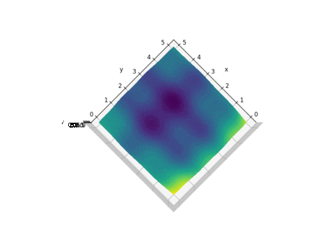
Plot of f(x,y)

As we can see from the plot above, this function looks like a curved egg carton. It is not a convex function and therefore it is hard to find its minimum because a local minimum found is not necessarily the global minimum.

So how can we find the minimum point in this function? For sure, we can resort to exhaustive search: If we check the value of $f (x, y)$ for every point on the plane, we can find the minimum point. Or we can just randomly find some sample points on the plane and see which one gives the lowest value on $f (x, y)$ if we think it is too expensive to search every point. However, we also note from the shape of $f (x, y)$ that if we have found a point with a smaller value of $f (x, y)$ , it is easier to find an even smaller value around its proximity.

This is how a particle swarm optimization does. Similar to the flock of birds looking for food, we start with a number of random points on the plane (call them particles) and let them look for the minimum point in random directions. At each step, every particle should search around the minimum point it ever found as well as around the minimum point found by the entire swarm of particles. After certain iterations, we consider the minimum point of the function as the minimum point ever explored by this swarm of particles.

Before we dive into our simple application case, let’s jump into the past. Particle Swarm Optimization is a population based stochastic optimization technique developed by Dr. Eberhart and Dr. Kennedy in 1995 [2] inspired by the social behavior of birds or schools of fish.

PSO traduction: a group of particles (potential solutions) of the global minimum in a research space. There is only a global minimum in this search space. None of the particles knows where the global minimum is located, but all particles have fitness values evaluated by the fitness function to be optimized.

Particle defined by its coordinates Particle Swarm Optimization (PSO) — Particle defined by its coordinates [Original Image]

Before going further in the explanation of the PSO algorithm, let’s focus a moment on our particles. As you will have understood, each of these particles is a potential solution of the function to be minimized. They are defined by their coordinates in the search space.

Random Initialization of particles position Particle Swarm Optimization (PSO) — Random Initialization of particles position [Original Image]

We can then randomly define particles in the search space as in the image above. But these particles must be in movement to find the optimal function.

Bedtime story: each of these birds moves with a certain speed of flight through the valley to find food.

PSO traduction: each of these particles is in movement with a velocity allowing them to update their position over the iterations to find the global minimum.

Particle velocity defined by the velocity in each direction Particle Swarm Optimization (PSO) — Particle velocity defined by the velocity in each direction [Original Image]

The particles have already been randomly distributed in the search space. Their velocity must then be initialized. Defined by its speed in each direction the velocity vector will once again be randomized. For this reason, we speak of stochastic algorithms.

Swarm

PSO shares many similarities with evolutionary computation techniques such as Genetic Algorithms (GA). The system is initialized with a population of random solutions and searches for optima by updating generations. However, unlike GA, PSO has no evolution operators such as crossover and mutation. The difference is in the way the generations are updated.

Bedtime story: while flying through the valley, the birds keep their speed (inertia) but also change their direction. Each bird aims to prove he is better than the others. He tries to find food based on his intuition (cognitive). But because he tends to imitate the others (social), he is also influenced by the experience and knowledge of his group.

PSO traduction: over the iterations in the search space, the speed of each particle is stochastically accelerated towards its previous best position (personal best) and towards the best solution of the group (global best).

Particle update Particle Swarm Optimization (PSO) — Particle update [Original Image]

Concretely, at each iteration, each particle is updated according to its velocity. This velocity is subject to inertia and is governed by the two best values found so far.

The first value is the best personal solution the particle has found so far. The second one is the best global solution that the swarm of particles has found so far. So each particle has in memory its best personal solution and the best global solution.

Optimization

As you might have noticed, I have not yet talked about the inertia, cognitive and social coefficients. These coefficients control the levels of exploration and exploitation. Exploitation is the ability of particles to target the best solutions found so far. Exploration, on the other hand, is the ability of particles to evaluate the entire research space. The challenge of the remaining part of the article will be to determine the impact of these coefficients to find a good balance between exploration and exploitation.

This assertion of a balance between exploration and exploitation does not make much sense unless both are defined in a measurable way and, moreover, such a balance is neither necessary nor sufficient from an efficiency point of view. But for the sake of understanding, I will use these terms in this article.

Bedtime story: each day, our emotionally driven birds can more or less get up on the wrong side of the bed. Then they will more or less want to follow their intuition and follow the group.

PSO traduction: at each iteration, the acceleration is weighted by random terms. Cognitive acceleration and social acceleration are stochastically adjusted by the weights r1 and r2.

Parameter tuning Particle Swarm Optimization (PSO) — Parameter tuning [Original Image]

These two weights r1 and r2 are unique for each particle and each iteration. This is not the case for the coefficients that I am going to introduce to you now.

Bedtime story: in wildlife, there are different bird species. These different species more or less like to change their direction over time.

PSO traduction: the hyperparameter w allows to define the ability of the swarm to change its direction. The particles have an inertia proportional to this coefficient w.

intertia weight Parameter tuning Particle Swarm Optimization (PSO) — w comparison [Original Image]

To better appreciate the influence of this coefficient w (also called inertia weight), I invite you to visualize the 3 swarms of particles above. We can then see that the lower the coefficient w, the stronger the convergence. In other words, a low coefficient w facilitates the exploitation of the best solutions found so far while a high coefficient w facilitates the exploration around these solutions. Note that it is recommended to avoid w >1 which can lead to a divergence of our particles.

The inertia weight w thus makes a balance between the exploration and the exploitation of the best solutions found so far. Let’s look at how these solutions are found by studying the coefficients c1 and c2 (also called acceleration coefficients).

Bedtime story: in wildlife, there are different bird species. Each species has an overall tendency to follow its instinct (personal) and a tendency to focus on the group experience (social).

PSO traduction: the c1 hyperparameter allows defining the ability of the group to be influenced by the best personal solutions found over the iterations. The hyperparameter c2 allows defining the ability of the group to be influenced by the best global solution found over the iterations.

c1 c2 coefficient Parameter tuning Particle Swarm Optimization (PSO) — c1 and c2 comparison [Original Image]

On the GIF above, we can see the impact of these two coefficients. For the purposes, I deliberately chose a very low coefficient w and forced the extremes of c1 and c2. We can notice then how the particles of the swarm are more individualistic when c1 is high. There is, therefore, no convergence because each particle is only focused on its own best solutions. In contrast, the particles of the swarm are more influenced by the others when c2 is high. We notice on the GIF that the exploration of the solutions is not optimal and that the exploitation of the best global solution is very important (this is obvious at iteration ~40).

The coefficients c1 and c2 are consequently complementary. A combination of the two increases both exploration and exploitation.

Auto hyperparameters

Bedtime story: defined as we just did, our bird species are a little weak-minded. What we would like is to have a group of birds that takes advantage of their numbers to explore the valley as well as possible. This same group of birds, after concertation, would exploit the best places by refocusing their search with their progress.

PSO traduction: we can go even further by updating coefficients over the iterations. Starting with a strong c1, strong w, and weak c2 to increase the exploration of the search space, we want to tend towards a weak c1, weak w, and strong c2 to exploit the best results after exploration by converging towards the global minimum.

Auto hyperparameters parameters Particle Swarm Optimization (PSO) — Auto hyperparameters over iterations [Original Image]

According to the paper by M. Clerc and J. Kennedy [3] to define a standard for Particle Swarm Optimization, the best static parameters are w=0.72984 and c1 + c2 > 4. More exactly c1 = c2 = 2.05. Additionally, the linear decay of the parameter w was initially proposed by Yuhui and Russ Y. H. Shi and R. C. Eberhart [4].

Based on these ideas and inspired by the paper by G. Sermpinis [1], I suggest the coefficients as specified in the image above.

For N iterations in total and t the current iteration, c2 grows linearly from 0.5 to 3.5 inversely to c1 which decreases from 3.5 to 0.5 to ensure c1 + c2 = 4. And w is initially 0.8 to slowly converges to 0.4.

Auto hyperparameters on Particle Swarm Optimization [Original Image]

Auto hyperparameters on Particle Swarm Optimization [Original Image]

Time Series Forecasting

Time series is a sequence of observations of categorical or numeric variables indexed by a date, or timestamp. A clear example of time series data is the time series of a stock price. In the following table, we can see the basic structure of time series data. In this case the observations are recorded every hour.

Timestamp	Stock - Price
2015-10-11 09:00:00	100
2015-10-11 10:00:00	110
2015-10-11 11:00:00	105
2015-10-11 12:00:00	90
2015-10-11 13:00:00	120

Normally, the first step in time series analysis is to plot the series, this is normally done with a line chart.

The most common application of time series analysis is forecasting future values of a numeric value using the temporal structure of the data. This means, the available observations are used to predict values from the future.

The temporal ordering of the data, implies that traditional regression methods are not useful. In order to build robust forecast, we need models that take into account the temporal ordering of the data.

The most widely used model for Time Series Analysis is called Autoregressive Moving Average (ARMA). The model consists of two parts, an autoregressive (AR) part and a moving average (MA) part. The model is usually then referred to as the ARMA(p, q) model where p is the order of the autoregressive part and q is the order of the moving average part.

Autoregressive Model

The AR(p) is read as an autoregressive model of order p. Mathematically it is written as −

X_{t} = c + \sum_{i = 1}^{P} ϕ_{i} X_{t - i} + ε_{t}

where {φ1, …, φp} are parameters to be estimated, c is a constant, and the random variable εt represents the white noise. Some constraints are necessary on the values of the parameters so that the model remains stationary.

Moving Average

The notation MA(q) refers to the moving average model of order q −

X_{t} = μ + ε_{t} + \sum_{i = 1}^{q} θ_{i} ε_{t - i}

where the θ1, ..., θq are the parameters of the model, μ is the expectation of Xt, and the εt, εt − 1, ... are, white noise error terms.

Autoregressive Moving Average

The ARMA(p, q) model combines p autoregressive terms and q moving-average terms. Mathematically the model is expressed with the following formula −

X_{t} = c + ε_{t} + \sum_{i = 1}^{P} ϕ_{i} X_{t - 1} + \sum_{i = 1}^{q} θ_{i} ε_{t - i}

We can see that the ARMA(p, q) model is a combination of AR(p) and MA(q) models.

To give some intuition of the model consider that the AR part of the equation seeks to estimate parameters for Xt − i observations of in order to predict the value of the variable in Xt. It is in the end a weighted average of the past values. The MA section uses the same approach but with the error of previous observations, εt − i. So in the end, the result of the model is a weighted average.

Examples of time series forecasting

Explore forecasting examples using InfluxDB, the open source time series database.

Storage forecasting

Here is a use case example of storage forecasting (at Veritas Technologies), from which the below screenshot is taken:

Storage Usage Forecast at Veritas Predictive Insights

Travelling Salesman Problem

Problem Statement

A traveler needs to visit all the cities from a list, where distances between all the cities are known and each city should be visited just once. What is the shortest possible route that he visits each city exactly once and returns to the origin city?

Solution

Travelling salesman problem is the most notorious computational problem. We can use brute-force approach to evaluate every possible tour and select the best one. For n number of vertices in a graph, there are (n - 1)! number of possibilities.

Instead of brute-force using dynamic programming approach, the solution can be obtained in lesser time, though there is no polynomial time algorithm.

Let us consider a graph G = (V, E), where V is a set of cities and E is a set of weighted edges. An edge e(u, v) represents that vertices u and v are connected. Distance between vertex u and v is d(u, v), which should be non-negative.

Suppose we have started at city 1 and after visiting some cities now we are in city j. Hence, this is a partial tour. We certainly need to know j, since this will determine which cities are most convenient to visit next. We also need to know all the cities visited so far, so that we don't repeat any of them. Hence, this is an appropriate sub-problem.

For a subset of cities S Є {1, 2, 3, ... , n} that includes 1, and j Є S, let C(S, j) be the length of the shortest path visiting each node in S exactly once, starting at 1 and ending at j.

When |S| > 1, we define C(S, 1) = ∝ since the path cannot start and end at 1.

Now, let express C(S, j) in terms of smaller sub-problems. We need to start at 1 and end at j. We should select the next city in such a way that

C (S, j) = m i n C (S - {j}, i) + d (i, j) w h e r e i \in S a n d i \neq j c (S, j) = m i n C (s - {j}, i) + d (i, j) w h e r e i \in S a n d i \neq j

Algorithm: Traveling-Salesman-Problem 
C ({1}, 1) = 0 
for s = 2 to n do 
   for all subsets S Є {1, 2, 3, … , n} of size s and containing 1 
      C (S, 1) = ∞ 
   for all j Є S and j ≠ 1 
      C (S, j) = min {C (S – {j}, i) + d(i, j) for i Є S and i ≠ j} 
Return minj C ({1, 2, 3, …, n}, j) + d(j, i)

Analysis

There are at the most $2^{n} . n$ sub-problems and each one takes linear time to solve. Therefore, the total running time is $O (2^{n} . n^{2})$

$O (2^{n} . n^{2})$

Thanks for reading the article. If you have any doubt or just wants to talk Data Science, write it in the comments below.

BDO PEER MENTOR